Introduction
The focus of this article is building a decision tree learner and evaluate its performance in different settings and finally compare it with a linear regression learner. The main learning goals are:
- Supervised Learning: Understanding what is supervised learning and how to train, query and evaluate its performance
- Decision Tree: Learning how to build a decision tree and use it in different configurations
Supervised Learning
Consider a series of predictor(here predictor just means inputs) measurements x_i, i = 1, 2, \dots, N where for each predictor there is an associated response measurement y_i. From a statistical point of view the goal is to usually find a fit such that we can relate the predictors to the responses as accurately as possible. This is interesting because it allows to understand the relationships between the predictors and responses and also we can use such a fit to make predictions of future values for responses given historical predictor data. Such problems where there is a series of predictor measurements and an accompanying series of response measurements belong to the supervised learning problems category.
The opposite of supervised learning problems are unsupervised learning where there is no associated series of response measurements for the predictors. This makes the learning problem more challenging as we are sort of working in blind. Another way to say this is that we do not have a response variable to supervise our analysis. This is where the terms supervised and unsupervised originate from.
CART Algorithms
Classification and Regression Trees (CARTs) algorithms are used in supervised machine learning to deduct information from large data sets for prediction purposes. In this article we will build a decision tree learner focused on regression analysis, meaning the data we will work with is numerical.
Decision Tree Learner
Our main learner is the decision tree learner based on JR Quinlan algorithm. The pseudocode of the algorithm is shown below.
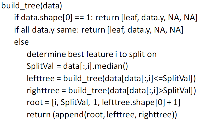
The algorithm build a decision tree in a recursive manner. In the actual implementation a hyperparameter called leaf size is also introduced which determines the aggregation threshold of the learner. The decision on what is the best feature to split on is made by computing the feature with the highest correlation coefficient.
We train our learner using financial stock market data. Our predictor measurements will be the adjusted closing price of different index funds and our goal is to provide a prediction for the MSCI Emerging Markets (EM) index. We will use 60% of the data set to train the learner and the other 40% is used to evaluate the predictions.
The implementation of our decision tree is given below.
class DTLearner:
"""
Decision Tree Learner
This class can be instantiated to create a decision learner for numerical analysis (regression)
Args:
leaf_size (int): the leaf size hyperparameter, used to decide the threshold of leaf aggregation
verbose (bool): toggle to allow printing to screen
Returns:
An instance of the class with a tree built from the data, the instance can then be used to query predictions
"""
def __init__(self, leaf_size=1, verbose=False):
self.leaf_size = leaf_size
self.verbose = verbose
self.tree = None
def add_evidence(self, data_x, data_y):
"""
Add training evidence
The method combines the separate data sets into one data set, this makes building the tree easier later.
Usually the shape of data_x is something like (r, c) and data_y is (r, ). We can combine this two data sets
if we concatenate along the axis for which the dimensions are not necessarily equal. But it is required to
first reshape data_y so that instead of a vector it becomes a 2-d array with a single column.
Args:
data_x (nd numpy array): a multidimensional numpy array holding the factor values
data_y (1d numpy array): a vector of labels (a.k.a. Y values)
Returns:
None, it just combines the data and invokes build_tree method
"""
data = np.concatenate((data_x, data_y[:, None]), axis=1)
self.tree = self.build_tree(data)
if self.verbose:
print(f'tree shape: {self.tree.shape}')
print(self.tree)
def find_best_feature(self, data):
"""
Find the best feature to split
It finds the best feature to split the rows using the correlation coefficient. We need to watch out
for the situation where the standard deviation of feature_x is zero, since this will result
in a division by zero in the calculation of the correlation coefficient and will cause a runtime error
Args:
data (nd numpy array): the data set as an n-dimensional numpy array
Returns:
The best feature to split the data on, the returned value is an integer representing the column index.
If there is a situation where the correlation coefficient for multiple columns are the same, it will
deterministicly return the last column.
"""
best_feature = None
best_corr_coef = float('-inf')
for col in range(data.shape[1] - 1):
feature_x = data[:, col]
# check std first, to prevent division by zero when numpy tries to
# calculate the covariance matrix
std = np.std(feature_x)
if std > 0:
c = np.corrcoef(feature_x, y=data[:, -1])[0, 1]
else:
c = 0
if c >= best_corr_coef:
best_corr_coef = c
best_feature = col
return best_feature
def build_tree(self, data):
"""
Builds the decision tree for numerical analysis based on the JR Quinlan algorithm
Args:
data (nd numpy array): the full data set as an n-dimensional numpy array
Returns:
The decision tree as a nd numpy array in a tabular format where each row is
[best_feature_idx, split_val, relative_left_tree_node_idx, relative_right_tree_node_idx]
A leaf can be determined when a given row has its best_feature_idx set to numpy nan.
"""
if data.shape[0] <= self.leaf_size:
return np.atleast_2d([np.nan, np.mean(data[:, -1]), np.nan, np.nan])
if np.all(data[:, -1] == data[0, -1]):
return np.atleast_2d([np.nan, data[0, -1], np.nan, np.nan])
best_feature_idx = self.find_best_feature(data)
split_val = np.median(data[:, best_feature_idx])
ys = data[:, best_feature_idx]
if np.all(ys <= split_val) or np.all(ys > split_val):
return np.atleast_2d([np.nan, np.mean(ys), np.nan, np.nan])
true_rows = data[data[:, best_feature_idx] <= split_val]
false_rows = data[data[:, best_feature_idx] > split_val]
left_tree = self.build_tree(true_rows)
right_tree = self.build_tree(false_rows)
root = np.atleast_2d([best_feature_idx, split_val, 1, left_tree.shape[0] + 1])
return np.vstack((root, left_tree, right_tree))
def predict(self, point, node=0):
"""
Predict the label for a given point
Args:
point (1d numpy array): 1 dimensional numpy array where each entry is the value for a feature
node (int): the current decision node
Returns:
A prediction for the label of a given point from the decision tree.
"""
if np.isnan(self.tree[node, 0]):
return self.tree[node, 1]
feature = int(self.tree[node, 0])
split_val = self.tree[node, 1]
if point[feature] <= split_val:
node += int(self.tree[node, 2])
else:
node += int(self.tree[node, 3])
return self.predict(point, node)
def query(self, points):
"""
Query the decision tree to get predictions for the given points
Args:
points (nd numpy array): nd numpy array where each entry is the value for a feature
Returns:
An 1d numpy array where each entry is the prediction for a given point
"""
predictions = np.empty([len(points), ])
for idx, point in enumerate(points):
predictions[idx] = self.predict(point)
return predictions
def print_tree(self, node=0, spacing=''):
"""
Print the decision tree
Args:
node (int): current node in the tree
spacing (str): current spacing
Returns:
None, it will just print the tree to the console
"""
if np.isnan(self.tree[node, 0]):
print(f'{spacing} Label: {self.tree[node, 1]}')
return
print(f'{spacing} <= {self.tree[node, 1]}')
print(f'{spacing} --> True:')
self.print_tree(int(self.tree[node, 2]) + node, f'{spacing}\t')
print(f'{spacing} --> False:')
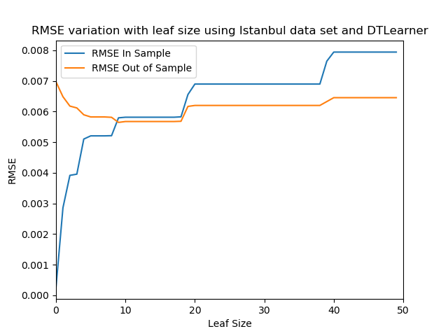
self.print_tree(int(self.tree[node, 3]) + node, f'{spacing}\t')We can experiment with our tree and evaluate its performance. In this experiment we train several instances of the decision tree learner by varying the leaf size. In each simulation we evaluate the performance of the learner by calculating the RMSE parameter for in sample and out of sample predictions.
def experiment_1(train_x, train_y, test_x, test_y):
    max_leaf_size = 50
    in_sample_rmse = np.empty([max_leaf_size, ])
    out_of_sample_rmse = np.empty([max_leaf_size, ])

    for leaf_size in range(1, max_leaf_size + 1):
        # create a learner and train it
        learner = dtl.DTLearner(leaf_size=leaf_size)
        learner.add_evidence(train_x, train_y)  # train it

        # evaluate in sample
        pred_y = learner.query(train_x)  # get the predictions
        rmse_in = math.sqrt(((train_y - pred_y) ** 2).sum() / train_y.shape[0])
        in_sample_rmse[leaf_size - 1] = rmse_in

        # evaluate out of sample
        pred_y = learner.query(test_x)  # get the predictions
        rmse_out = math.sqrt(((test_y - pred_y) ** 2).sum() / test_y.shape[0])
        out_of_sample_rmse[leaf_size - 1] = rmse_out

    df_temp = pd.concat(
        [pd.DataFrame(in_sample_rmse).rename(columns={0: 'RMSE In Sample'}), pd.DataFrame(out_of_sample_rmse).rename(columns={0: 'RMSE Out of Sample'})], axis=1
    )
    df_temp.plot()

    plt.title('RMSE variation with leaf size using Istanbul data set and DTLearner')
    plt.xlabel('Leaf Size')
    plt.ylabel('RMSE')

    plt.xlim((0, 50))
    plt.savefig('./experiment_1.png')
The result of the experiment can be seen in the figure below. When evaluating the performance of our learner we are interested in whether overfitting occurs or not. Overfitting is an undesirable situation where a learner tries to fit the training data excessively, in other words the learner simply overlearns the training data. As a result, the learner is unable to handle test data properly and provide accurate estimates.
Looking at the figure, it can be seen overfitting occurs for a leaf size < 10. In this range, the RMSE for in sample data, i.e. training data, is increasing with leaf size, while the RMSE for out of sample data, i.e. test data, is decreasing with leaf size. When leaf size increases the flexibility of the learner decreases, at low leaf sizes the learner will fit almost one-to-one to the training data, this explains the in-creasing behavior of the in sample data RMSE, as the learner is forced to aggregate leaves, its prediction accuracy decreases. On the other hand, the test data RMSE is decreasing because, by increasing the leaf size the learner is forced to generalize. As leaf size approaches 10, the RMSE seems to be optimum for in sample and out of same. For leaf size > 10 both in sample and out of sample RMSE seems to be increasing, meaning the learner’s ability to provide accurate estimates is decreasing.