Introduction
This article is about using Python to analyze portfolio stocks and allocations. The primary learning goals are:
- Portfolio Analysis: Given a portfolio of stocks implement several metrics to evaluate the performance of a portfolio
Portfolio Analysis
There are several metrics that can be used to evaluate the performance of a portfolio. Here we focus on the metrics below:
- Daily Returns: How much a price went up or down on a particular day
- Cumulative Return: A measure of how much the value of the portfolio has gone up from the beginning to the end
- Average Daily Return: Simply the mean of the daily returns
- Standard Deviation of Daily Return: Simply the standard deviation of the daily returns
- Sharpe Ratio: Risk adjusted return
Sharpe Ratio (SR)
A measure that adjusts returns for risk. All else being equal, lower risk is better, higher returns is better. Also, SR takes into account the risk free rate of return. This is the return one would get if they invested their capital in short term treasury or bank account. However, this value has been almost zero since 2015.
To compute the Sharpe Ratio the equation below can be used.
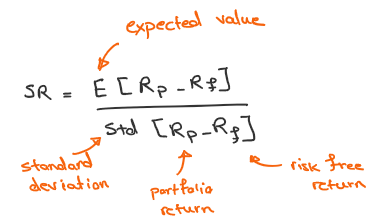
From statistics we know that we can calculate the expected value of a series by simply taking the mean of the series. Sharpe ratio is highly dependent on how frequently sampling is done. SR is usually an annual measure and we can normalize it by using a coefficient that depends on the sampling frequency.
Implementation
We start implementing the portfolio analysis metrics for a set of stock symbols. Our goal is to write the code in such a way that any number of stock symbols are supported.
To calculate anything data is needed, either as local files in a CSV format or downloading them online, manually or through a package such as yfinance. One way or another, we assume data is available and it is has the following structure.
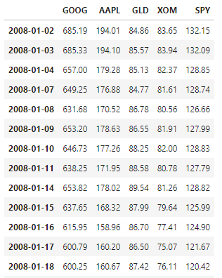
The rows or the index are datetimes and the columns are the prices for the symbols. We use SPY (S&P 500) symbol as a sort of reference frame to make comparisons with.
First step is to calculate the portfolio daily value. We assume no changes will occur on day 1 and that there will be only changes on a daily basis. The function below calculates the portfolio daily value.
def compute_portfolio_daily_value(prices, allocs, sv):
"""
Compute portfolio daily value
Args:
prices (DataFrame): A n*m pandas dataframe where n is an index of dates and m is a set of stock symbol prices
allocs (list): A 1-d list of initial stock allocation, it must sum to 1
sv (integer): Starting value of the portfolio
Returns:
A 1-d pandas dataframe where each entry is the value of the portfolio indexed by day.
"""
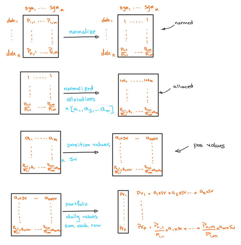
normed = prices / prices.values[0]
alloced = normed.multiply(allocs)
pos_vals = alloced.multiply(sv) # alloced * start_val
port_val = pos_vals.sum(axis=1) # the daily value of the portfolio
return port_valSo, there are a couple of things happening here, the end goal is to calculate the daily value of the portfolio, and to get there several operations are performed on the data which is explained below.
Once the portfolio daily value is computed, it is possible to determine the daily return value, a very important metric in portfolio analysis.
def compute_portfolio_daily_returns(port_val):
    """
    Compute portfolio daily returns

    Args:
        port_val (DataFrame): A 1-d pandas dataframe where each entry is the value of the portfolio indexed by day

    Returns:
        A 1-d pandas dataframe where each entry is the daily return value of the portfolio indexed by day
    """
    daily_returns = (port_val / port_val.shift(1)) - 1
    daily_returns = daily_returns[1:]  # Pandas leaves the 0th row full of NaNs, read this as dropping row 0 across all columns

    return daily_returns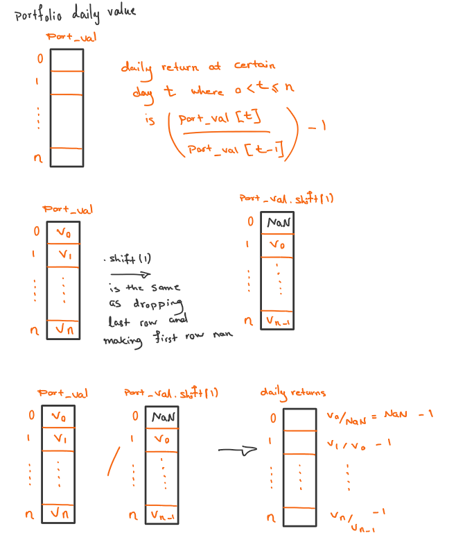
Finally it is now possible to calculate the rest of the important metrics of the portfolio to evaluate its performance.
def compute_portfolio_stats(port_val, daily_returns, sf, rfr):
    """
    Compute portfolio statistics

    Args:
        port_val (DataFrame): A 1-d pandas dataframe where each entry is the value of the portfolio indexed by day
        daily_returns (DataFrame): A 1-d pandas dataframe where each entry is the daily return value of the portfolio indexed by day
        sf (float): Sampling frequency, daily=252, weekly=52, monthly=12
        rfr (float): Risk free return rate

    Returns:
        A tuple (cum_ret, avg_daily_ret, std_daily_ret, sr) where cum_ret is the cumulative return, avg_daily_ret is the average daily return,
        std_daily_ret is the standard deviation of the daily return and sr is the sharpe ratio
    """
    cum_ret = (port_val[-1] / port_val[0]) - 1
    avg_daily_ret = daily_returns.mean()
    std_daily_ret = daily_returns.std()
    sr = math.sqrt(sf) * (daily_returns - rfr).mean() / daily_returns.std()

    return cum_ret, avg_daily_ret, std_daily_ret, sr
Putting it all together, the code below handles the computation and optionally generates a plot in comparison with SPY symbol.
import datetime as dt
import pandas as pd
import math
import matplotlib.pyplot as plt
from util import get_data
def compute_portfolio_daily_value(prices, allocs, sv):
"""
Compute portfolio daily value
Args:
prices (DataFrame): A n*m pandas dataframe where n is an index of dates and m is a set of stock symbol prices
allocs (list): A 1-d list of initial stock allocation, it must sum to 1
sv (integer): Starting value of the portfolio
Returns:
A 1-d pandas dataframe where each entry is the value of the portfolio indexed by day.
"""
normed = prices / prices.values[0]
alloced = normed.multiply(allocs)
pos_vals = alloced.multiply(sv) # alloced * start_val
port_val = pos_vals.sum(axis=1) # the daily value of the portfolio
return port_val
def compute_portfolio_daily_returns(port_val):
"""
Compute portfolio daily returns
Args:
port_val (DataFrame): A 1-d pandas dataframe where each entry is the value of the portfolio indexed by day
Returns:
A 1-d pandas dataframe where each entry is the daily return value of the portfolio indexed by day
"""
daily_returns = (port_val / port_val.shift(1)) - 1
daily_returns = daily_returns[1:] # Pandas leaves the 0th row full of NaNs, read this as dropping row 0 across all columns
return daily_returns
def compute_portfolio_stats(port_val, daily_returns, sf, rfr):
"""
Compute portfolio statistics
Args:
port_val (DataFrame): A 1-d pandas dataframe where each entry is the value of the portfolio indexed by day
daily_returns (DataFrame): A 1-d pandas dataframe where each entry is the daily return value of the portfolio indexed by day
sf (float): Sampling frequency, daily=252, weekly=52, monthly=12
rfr (float): Risk free return rate
Returns:
A tuple (cum_ret, avg_daily_ret, std_daily_ret, sr) where cum_ret is the cumulative return, avg_daily_ret is the average daily return,
std_daily_ret is the standard deviation of the daily return and sr is the sharpe ratio
"""
cum_ret = (port_val[-1] / port_val[0]) - 1
avg_daily_ret = daily_returns.mean()
std_daily_ret = daily_returns.std()
sr = math.sqrt(sf) * (daily_returns - rfr).mean() / daily_returns.std()
return cum_ret, avg_daily_ret, std_daily_ret, sr
def assess_portfolio(
symbols,
allocs,
sd=dt.datetime(2008, 1, 1),
ed=dt.datetime(2009, 1, 1),
sv=1000000,
rfr=0.0,
sf=252.0,
gen_plot=False
):
"""
Calculate portfolio assessment metrics
Args:
symbols (list): A list of stock symbols
allocs (list): A list of initial stock allocations, must sum to 1
sd (datetime): Starting datetime
ed (datetime): Ending datetime
sv (integer): Starting value of the portfolio
rfr (float): Risk free return rate
sf (float): Sampling frequency, daily=252, weekly=52, monthly=12
Returns:
A tuple (cr, adr, sddr, sr) where cr is the cumulative return, adr is the average daily return,
sddr is the standard deviation of the daily return and sr is the sharpe ratio
"""
prices_all = get_data(symbols=symbols, dates=(sd, ed))
prices = prices_all[symbols]
prices_SPY = prices_all['SPY']
port_val = compute_portfolio_daily_value(prices, allocs, sv)
daily_returns = compute_portfolio_daily_returns(port_val)
cr, adr, sddr, sr = compute_portfolio_stats(port_val, daily_returns, sf, rfr)
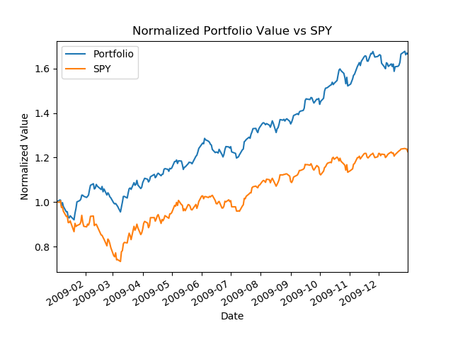
if gen_plot:
df_temp = pd.concat(
[port_val / port_val[0], prices_SPY / prices_SPY[0]],
keys=['Portfolio', 'SPY'],
axis=1
)
df_temp.plot()
plt.xlabel('Date')
plt.ylabel('Normalized Value')
plt.title('Normalized Portfolio Value vs SPY')
plt.savefig('./analysis.png')
return cr, adr, sddr, sr
if __name__ == '__main__':
assess_portfolio(
symbols=['GOOG', 'AAPL', 'GLD', 'XOM'],
allocs=[0.2, 0.3, 0.4, 0.1],
sd=dt.datetime(2009, 1, 1),
ed=dt.datetime(2010, 1, 1),
gen_plot=True
)Using the sample inputs in the code above, the generated plot would look like the following.